
Information Theory of Deep Learning
EDIT: I have moved to Substack and I regularly blog there. Click here to subscribe for great content on productivity, life and technology.
In this post, I will try to summarize the findings and research done by Prof. Naftali Tishby which he shares in his talk on Information Theory of Deep Learning at Stanford University recently. There have been many previous versions of the same talk so don’t be surprised if you have already seen one of his talks on the same topic. Most of the summary will be based on his research and I will try to include some relevant mathematics (not everything) for better understanding of the concepts. I will assume some knowledge of basic deep learning and neural networks along with some familiarity with the fundamentals of machine learning (mostly supervised learning). This post will summarize most of his research on the topic till now and hence, will be a bit longer but it is going to be a fun read! So let’s move forward with it!
Motivation
If you have tried understanding the math behind a lot of deep learning concepts, I am sure you must have come across some topics from information theory such as the Kullback-Leibler divergence (aka. KL divergence), Jensen-Shannon divergence, Shannon entropy, etc. For me, I came across these terms too many times to not write about them, especially while studying generative models such as Restricted Boltzmann Machines and General Adversarial Networks. While searching on the topics I came across this great talk by Prof. Tishby which captured my attention and made me think about deep neural networks with a totally different perspective. So I decided to research his findings and discover this new angle of looking at the working of DNNs. I enjoyed reading the topic so much that I decided to write a blog post to document his findings and my learnings so that it might help someone like you who might want to learn about it in a shorter amount of time. The motivation to write this post started from knowing about different information theory measures used in deep learning but I ended up reading much more and learned a lot of exciting stuff that I am eager to share with you. Note that I am new to information theory and learning theory and therefore, there may be places where things are not so clear (expect some rough edges). So without wasting any more mental energy, let’s move on to the discussion on Information Theory!
Information Theory
Before diving into the relevance of this topic in deep learning, let us first try to understand what information theory is and what is it used for.
Information theory is based on probability theory and statistics and often concerns itself with measures of information of the distributions associated with random variables. Important quantities of information are entropy, a measure of information in a single random variable, and mutual information, a measure of information in common between two random variables. Information theory revolves around quantifying how much information is present in a signal. It was originally invented to study sending messages from discrete alphabets over a noisy channel, such as communication via radio transmission. The basic intuition behind information theory is that learning that an unlikely event has occurred is more informative than learning that a likely event has occurred. In the case of deep learning, the most common use case for information theory is to characterize probability distributions and to quantify the similarity between two probability distributions. We use concepts like KL divergence and Jensen-Shannon divergence for these purposes.
Basic Concepts
Note: Not all of these concepts are used in Prof. Tishby’s work but I decided to include them anyway as they are a part of Information Theory and are often used in Deep Learning.
1. Entropy
The Shannon entropy H, in units of bits (per symbol) is given by
\[H = -\displaystyle \sum_i p_i \, \log_2 (p_i)\]where \(p_i\) is the probability of occurrence of the \(i_{th}\) possible value of the source symbol. Intuitively, the entropy \(H_X\) of a random variable \(X\) gives us a measure of the amount of uncertainty associated with the value of X when only its distribution is known. Below is an example of the entropy of a Bernoulli trial as a function of the success probability (called the binary entropy function):

Fig.1 Entropy \(Η(X)\) (i.e. the expected surprisal) of a coin flip, measured in bits, graphed versus the bias of the coin \(Pr(X = 1)\), where \(X = 1\) represents a result of heads. (Image Source: Wikipedia page on Entropy)
We can see that this function is maximized when the two possible outcomes are equally probable, for example, like in an unbiased coin toss. In general for any random variable \(X\), the entropy \(H\) is defined as
\[H(X)=\mathbb {E}_{X}[I(x)]= - \displaystyle \sum_{x \in \mathbb{X}} p(x)\log p(x)\]where \(\mathbb{X}\) is the set of all messages \(\{x_1, ..., x_n\}\) that \(X\) could be and \(I(x)\) is the self-information, which is the entropy contribution of an individual message. As is evident from the Bernoulli case above, the entropy of a space is maximized when all the messages in the space are equally probable.
2. Joint Entropy
This concept of entropy applies when there are two random variables (say \(X\) and \(Y\)). The joint probability of \((X, Y)\) is defined as:
\[H(X,Y)=\mathbb {E}_{X,Y}[-\log p(x,y)]= - \displaystyle \sum_{x,y}p(x,y)\log p(x,y)\,\]This entropy is equal to the sum of the individual entropies of \(X\) and \(Y\) when they are independent. I am sure you might have heard about cross entropy a lot while studying loss functions and optimization in deep learning and I want to emphasize that it is different from joint entropy and you should not confuse the joint entropy of two random variables with cross entropy.
3. Conditional Entropy
The conditional entropy (also called conditional uncertainty) of a random variable \(X\) given a random variable \(Y\) is the average conditional entropy over \(Y\):
\[{\displaystyle H(X\mid Y)=\mathbb {E}_{Y}[H(X\mid y)]=-\sum_{y\in Y}p(y)\sum_{x\in X}p(x\mid y)\log p(x\mid y)=-\sum_{x,y}p(x,y)\log p(x\mid y)}\]One basic property that the conditional entropy satisfies is given by:
\[H(X\mid Y)=H(X,Y)-H(Y)\,\]4. Mutual Information
Using mutual information, we can quantify the amount of information that can be obtained for one random variable using the information from the other. The mutual information of X relative to Y is given by:
\[{\displaystyle I(X;Y)=\mathbb {E}_{X,Y}[SI(x,y)]=\sum_{x,y}p(x,y)\log {\frac {p(x,y)}{p(x)\,p(y)}}}\]where \(SI(x,y)\) is the Specific Mutual Information (also called pointwise mutual information) and is defined as:
\[\operatorname {pmi} (x;y)\equiv \log {\frac {p(x,y)}{p(x)p(y)}}=\log {\frac {p(x\mid y)}{p(x)}}=\log {\frac {p(y\mid x)}{p(y)}}\]A basic property of the mutual information is that
\[{\displaystyle I(X;Y)=H(X)-H(X\mid Y)\,}\]Intuitively, this means that knowing \(Y\), we can save an average of \(I(X; Y)\) bits in encoding \(X\) compared to not knowing \(Y\).
Mutual information is symmetric:
\[{\displaystyle I(X;Y)=I(Y;X)=H(X)+H(Y)-H(X,Y).\,}\]5. Kullback–Leibler divergence (information gain)
KL divergence is used to compare two probability distributions over the same random variable \(X\) and it tells us how different these two distributions are.
It is given by:
\[D_{\mathrm {KL}}(p(X)\mid q(X)) = \mathbb{E}_{x \sim P} \Big[\log \frac{P(x)}{Q(x)} \Big]\] \[= \displaystyle \sum_{x\in X}p(x)\log {\frac {p(x)}{q(x)}}\] \[= \mathbb{E}_{x \sim P} [\log P(x) - \log Q(x)]\] \[= \displaystyle \sum_{x\in X} p(x)\log {p(x)}\,-\,\sum_{x\in X}p(x)\log {q(x)}\]Note that KL divergence has some important properties like:
- it is non-negative.
- it is non-symmetric.
Due to the non-symmetric nature, KL divergence is not a true distance measure between the two distributions. For more information and a better understanding of all of these basic concepts, refer to this wikipedia page on information theory.
6. Jensen-Shannon Divergence
Jensen-Shannon Divergence is a smoother and symmetric version of measuring the similarity between two probability distributions and it is bounded by \([0,1]\).
\[D_{JS}(p\mid \mid q) = \frac{1}{2}D_{KL}(p\mid \mid \frac{p+q}{2})+\frac{1}{2}D_{KL}(q\mid \mid \frac{p+q}{2})\]
Fig.2 Jensen-Shannon divergence, which is symmetric as opposed to KL divergence which is non-symmetric. \(p\) and \(q\) are two Gaussian distributions with mean \(0\) and variance \(1\), \(m\) is the average of the two \((p+q)/2\) (Image Source: Lilian Weng’s blog post on WGANs vs GANs)
7. Markov Chain
A Markov property (also called the memoryless property) of a stochastic process refers to the dependence of conditional probability distributions of future states of the process only on the present states and not on the past states. A process with this property is called a Markov process. A Markov Chain is a type of Markov process that has a discrete state space.
8. Data Processing Inequality
For any Markov chain: \(X \rightarrow Y \rightarrow Z\), we would have \(I(X;Y)≥I(X;Z)\) A deep neural network can be viewed as a Markov chain where information is passed from one layer to the next, and thus when we are moving down the layers of a DNN, the mutual information between the layer and the input can only decrease.
9. Reparametrization invariance
For two invertible functions \(\phi\), \(\psi\), the mutual information still holds: \(I(X;Y)=I(\phi(X);\psi(Y))\).
In DNN context, this means that if we shuffle the weights in one layer of DNN, it would not affect the mutual information between this layer and the other layers. This is bad news for anyone who is trying to use mutual information to calculate the computational complexity because this means creating any hard to invert transformation of our data would not affect the information measures but it will increase the computational complexity greatly.
Now that we have summarized all the relevant terms and concepts to get familiar with information theory, let us move on to the task of linking this to deep learning and how it might be useful in the field.
Information Theory in Deep Learning
Introduction
With the advent of deep learning as the best performing technique on real data challenges and most of the supervised learning tasks, this new field is revolutionizing the tech world at a very fast pace. Most of the people are learning how to apply and use it without learning about the theoretical understanding of the concepts in DL. In order to try and understand this theory behind the working of these algorithms, we need to formulate deep learning as an information theoretic tradeoff between compression and prediction.
The above idea can be seen in the following way. The goal of any supervised learning algorithm (we will talk only about basic supervised learning using deep feed-forward networks here) is to capture as much relevant information as possible from the input variables about the output variable. This means extracting an appropriate minimum sufficient statistics of the input with respect to the output which in case of information theory, means to use a principled way to find a maximally compressed mapping of the input variable that preserves as much information as possible about the output variable. This concept is explained by Prof. Tishby in terms of the Information Bottleneck Principle that we will talk about a little later.
Deep Neural Networks: an Information Theoretical perspective
Our goal in supervised learning is to find a good representation \(T(x)\) of the input patterns \(x\), so that it enables a good prediction of the output label \(y\). In order to do this, we want an efficient way to learn the patterns from the (unknown) joint distribution \(P(X,Y)\) that also gives a good generalization. In general supervised learning using deep neural networks, the input variable is generally much higher in dimensionality as compared to the output variable. This generally means that most of the entropy of \(X\) is not very informative about \(Y\), and that the relevant features in \(X\) are highly distributed and difficult to extract. The remarkable success of deep learning algorithms in extracting such relevant features lies in their architecture involving multiple layers to process sequential information in which each hidden layer helps in extracting some information which is then passed on to the next layer and a higher level distributed representation is learned in the process. The goal is to statistically decouple input units without the loss of relevant information. Single neurons in DNN architectures can (usually) only classify linearly separable inputs as they can implement only hyperplanes in their input space \(\big(\boldsymbol{u = w·h+b}\big)\). Hyperplanes can optimally classify data when the inputs are conditionally independent. As conditional independence cannot be assumed for general data distributions, representational changes through the hidden layers are required, up to linear transformation that can decouple the inputs. The analysis done by Tishby et al. suggests that the optimal DNN architecture is determined solely by an information theoretic analysis of the joint distribution of the data, \(p(X,Y)\).
The Information Bottleneck Method
The information bottleneck method is an information theoretic principle for extracting relevant information that an input variable \(X\) contains about an output variable \(Y\). Given their joint distribution \(P(X,Y)\), the relevant information is defined as the mutual information \(I(X;Y)\). We assume a statistical dependence between \(X\) and \(Y\) and \(Y\) implicitly determines the relevant and irrelevant features in \(X\). an optimal representation \(\hat{X}\) of \(X\) would capture all the relevant information that is useful in the prediction of \(Y\) and discard all the other non-useful information.
Optimally, DNNs should learn to extract the most efficient informative features, or approximate minimal sufficient statistics, with the most compact architecture (i.e. minimal number of layers, with a minimal number of units within each layer).
Information Characteristics of DNN layers

Fig.3 A feedforward deep neural network architecture with \(m\) hidden layers, X is the input, Y is the output and \(\hat{Y}\) is the predicted output. The hidden layers form a Markov chain, \(I(Y ; \hat{Y} )/I(X; Y )\) quantifies how much of the relevant information is captured by the network. (Image Source: Tishby and Zaslavsky, 2015)
As can be seen from the DNN architecture above, the layers in the DNN form a Markov chain. This is because any layer in the network can take as input only the information output from the previous layer. This interpretation clearly shows that if some information about \(Y\) is lost in one hidden layer, it cannot be recovered in further hidden layers as the next hidden layer depends on the previous layers for their input. In mathematical terms, this means that for any hidden layer \(h_i\) and \(h_j\) where \(i \geq j\), the following property holds.
\[I(X; Y) \geq I(h_j; Y) \geq I(h_i; Y) \geq I(\hat{Y}; Y)\]We now define a quantity called the expected IB (Information Bottleneck) distortion which is given by
\[D_{IB} = E \big[d_{IB}(X, \hat{X}) \big] = I(X; Y \mid \hat{X})\]which is the residual information between \(X\) and \(Y\), which means the information that is not captured by \(\hat{X}\). The information distortion of the IB principle provides a new measure of optimality which can be applied not only for the output layer, as done when evaluating the performance of DNNs with other distortion or error measures, but also for evaluating the optimality of each hidden layer or unit of the network. This gives us an important measure of optimality because other cost functions such as the squared error cannot help in measuring the optimality of the hidden layers.
The analysis done by Prof. Tishby et al. in this paper shows that even though the input layer of a network contains more information about the target variable \(Y\), it is not good for generalization because the representation is too complex. So in order to get a good generalization, we also need a good amount of compression. In other words, the hidden layers must compress the input in order to reach a point where the worst case generalization error is tolerable.

Fig.4 A qualitative information plane with theoretical and practical IB limits. The black line is the optimal achievable IB limit, and the blue lines are sub-optimal IB bifurcations, obtained by forcing the cardinality of \(\hat{X}\) or remaining in the same representation. The red line corresponds to the upper bound on the out-of-sample IB distortion (mutual information on \(Y\)), when training from a finite sample. (Image Source: Tishby and Zaslavsky, 2015)
This is an image of a qualitative information plane with the x and the y-axes representing the complexity and the expected distortion respectively. In mathematical terms, the coordinates can be seen as \(I(X; T)\) and \(I(T; Y)\) where \(T(x)\) is an internal representation of the input \(X\). The black line gives the optimal achievable IB limit, the red line gives the upper bound on the out-of-sample IB distortion with a finite sample. The blue lines represent sub-optimal IB bifurcations that can be obtained by putting restrictions on the cardinality of \(\hat{X}\). The green line shows the path that might actually be followed when learning using a DNN. What it shows is consistent with the results we discussed above. It shows that $X$ contains the least amount of distortion but is the most complex representation without any compression and therefore, would not generalize well. The generalization error is dominated by the Y-axis which is the information about the label (higher the information, smaller the error). The X-axis dominates the number of examples that we need (sample complexity) and gives us an idea of how much we forget about the input in bits.
As we move forward through the hidden layers, we slowly reach the optimal line with the finite sample after possibly pruning irrelevant information from X and thus compressing the representation but increasing the distortion in the process. The terms \(\Delta C\) and \(\Delta G\) show us the generalization gap and the complexity gap which help us determine the performance of the network in terms of prediction and compression. The goal of the network then is to optimize the Information Bottleneck (IB) tradeoff between compression and prediction, successively, for each layer. In our case, \(\frac{I(Y; \hat{Y})}{I(X; Y)}\) will quantify how much of the relevant information is captured by the network.
Opening the black box of DNNs via Information

Fig.5 A DNN architecture visualized as encoder and decoder. Any representation of the input, \(T\), is defined through an encoder, \(P(T\mid X)\), and a decoder \(P(\hat{Y} \mid T)\), and can be quantified by its information plane coordinates: \(I_X = I(X; T)\) and \(I_Y = I(T; Y)\). (Image Source: Tishby and Schwartz-Ziv, 2015)
As described earlier, deep neural networks can be considered as a Markov chain of successive representations of input where information is flowing from one hidden layer to the next. Another way to look at the network is using the view above in which we consider the layers in terms of an encoder \(P(T\mid X)\) and a decoder \(P(Y\mid T)\) where the encoder tries to encode the input \(X\) into a compressed representation \(T\) and then the decoder will try to extract the information about the label \(Y\) using the information present in \(T\). This view is quite similar to how autoencoders work. Near the first hidden layer, the encoder is simple but the decoder is complicated. As we move towards the last hidden layer, the encoder becomes more and more complex and the decoder becomes simpler. The only two parameters that are important in this scenario are the mutual information of the encoder and the decoder (which are the axes of our information plane). We quantify in this way so as to take the advantage of the invariance of any invertible re-parametrization of T. Moving forward, we will look at some aspects of Stochastic Gradient Descent (SGD) and learn how it can help achieve optimal representations (a minimal sufficient statistic of \(X\) with respect to \(Y\) - if such can be found) that we saw on the Information Bottleneck curve.
For the \(m\)-layered DNN architecture using the DPI order as shown in the diagram, we have
\[I(X; Y) ≥ I(T_1; Y) ≥ I(T_2; Y) ≥ ... ≥ I(T_m; Y) ≥ I(\hat{Y} ; Y)\]and
\[H(X) ≥ I(X; T_1) ≥ I(X; T_2) ≥ ... ≥ I(X; T_m) ≥ I(X; \hat{Y} )\]These inequalities imply that the information about both the input and desired output decreases as we move forward through the layers due to the DPI property. This is a unique information path for the network formed by \(m\) monotonic points on the information plane. Each point on the plane corresponds to different possible DNN architectures as the same points are obtained after re-parametrization using any invertible function.
Schwartz-Ziv and Tishby emphasize the fact that a little noise in the function mapping from the input to the output helps in understanding machine learning complexity using information measures. They say that for deterministic functions \(y = f(x)\), the mutual information is insensitive to the complexity of the function \(f(x)\). The cure for this problem comes from the noise that is added to the patterns using stochastic versions of the functions (for a simple example, like using the sigmoid function in a perceptron to output the conditional probabilities \(p(y \mid x)\) instead of the class itself). Without the stochastic spread of the sigmoid output the mutual information is simply the entropy \(H(Y)\) independent of the function \(f(x)\), and there is nothing in the structure of the points \(p(y\mid x)\) on the simplex \([0,1]\) to hint to the geometry or learning complexity of the rule.
To compare different DNN architectures in terms of their efficiency to preserve relevant information in the joint distribution of \(X\) and \(Y\), we can visualize them on the information plane using the parameters \(I(T; X)\) and \(I(T; Y)\) and explore the effect of different parameters in the training process and the architecture through experiments.
Two Optimization Phases
We now talk about the two observed phases during the optimization process using SGD, namely the drift and the diffusion phase. Below is an image of the snapshots of the information plane for three different stages during the SGD optimization process. The left one is the initial stage of the weights, the center one is the situation after 400 epochs and the right one after 9000 epochs. The colors signify the different hidden layers (orange one being the farthest from the input layer) and the points correspond to 50 different random initializations. Note that the last hidden layer lies to the lower left in the plane because it contains very little information about both the input and the output.

Fig.6 A snapshot of the layers of the network on the information plane during SGD optimization (left - initial weights, mid - after 400 epochs, right - after 9000 epochs). The different points correspond to 50 different weight initializations. (Image Source: Tishby and Schwartz-Ziv, 2015)
- The first phase is explained by the cross-entropy loss minimization during which the layers increase the information on the labels as well as the input while preserving the Data Processing Inequality order (lower layers have higher information).
- The second phase is a little mysterious as the compression that can be seen taking place is not because of any explicit regularization or a related technique. This phase is a lot slower as compared to the first phase and the layers lose irrelevant information during this phase until convergence.
Here is a GIF of the process in action:
For a full video of the process in action, visit this link. The convergence is really beautiful! Now we will look at the effect of different number of training examples on the convergence on the information plane.
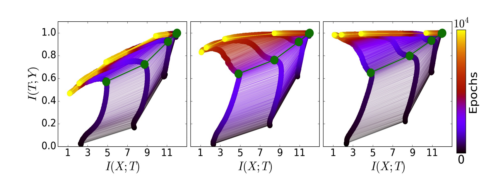
Fig.7 The evolution of the layers with the training epochs in the information plane, for different training samples. On the left - 5% of the data, middle - 45% of the data, and right - 85% of the data. The colors indicate the number of training epochs with Stochastic Gradient Descent from 0 to 10000 epochs. (Image Source: Tishby and Schwartz-Ziv, 2015)
The above picture shows these two phases converging to different positions on the information plane for different training samples which are 5%, 45% and 85% from left to right. The colors indicate the number of training epochs with Stochastic Gradient Descent from 0 to 10000. The green paths mark the distinction between the drift and the diffusion phases. As can be seen in the picture, less number of training examples lead to convergence very far from the convergence with more number of examples in the data. The label information is reduced in the case with less number of examples during the compression phase. In this case, we are overcompressing to the point that the representation is now too simple to capture the label information. In the case with a large number of samples, on the other hand, the label information is clearly increasing during the compression phase. Now we will look at a better explanation of what actually happens during these two phases by examining the behavior of stochastic gradients along the epochs.
Diffusion and Drift Phases
The number of epochs that the training process takes in order to reach the green path boundary is very less when compared to the total number of epochs or the number of epochs needed in the compression phase. The training error reduces to a very small quantity at this point after which the diffusion phase starts in which the noise in the gradient dominates the training process. Tishby calls this phase as the forgetting phase and argues that it is the most important phase in the learning process as the model learns to forget. This can be bolstered by the fact that even though all the fitting of the data happens in the first phase, most of the information gain about the label happens in the second phase. Most of the irrelevant information about the patterns is discarded in this phase and this results in an overall compression.

Fig.8 The mean and the standard deviation of the gradients during the SGD optimization process as a function of training epochs in log-log scale. The grey line marks the transition phase from drift to diffusion. (Image Source: Tishby and Schwartz-Ziv, 2015)
The network shown in the above picture is the architecture used in this experiment but the results obtained apply to any general deep network in the same way. The grey line in the graph marks the beginning of the dominance of the standard deviation over the mean of the gradient. In the second phase, the gradient is very noisy and results in the addition of random noise to the weights. The analysis in the information theoretical perspective is consistent with the solution to a Fokker-Plank equation without any information theory which gives the same story. This strengthens Tishby’s claim that this is the most important phase of learning. All this is possible because of the fluctuations in the mini-batches and changing the size of mini-batches shows that the point where the compression starts is exactly linearly related to the phase transition point in the gradient. Some compression is seen even with a full batch training.
One thing to note here is that there is no correlation between the weights or the neurons in the layers in the experiment but still we see a sharp convergence in all the different random initializations. Tishby says that this is what we desire (thing getting concentrated in large limits) and it happens when we have good order parameters.

Fig.9 The average trajectory of the hidden layers during the optimization process on the information plane. (Image Source: Quantamagazine’s post on the theory by Tishby et al.)
The image above shows the trajectory that the hidden layers follow (the different random initializations are averaged to get the trajectory of each hidden layer). The trajectory from A to C is fitting the data and from C to E is the generalization. Note that all the layers reach the inflection point C more or less together.

Fig.10 The average trajectory of the hidden layers during the optimization process on the information plane and the gradient information for a non-symmetric rule and architecture. This is consistent with the findings for a symmetric architecture. (Image Source: Tishby and Schwartz-Ziv, 2015)
For the following section, I will try to explain some bits of the learning theory as explained by Tishby in his talk but I must admit that I am far from an expert in learning theory (in fact I am just a beginner), so expect some rough edges here and there in the explanation.
Learning Theory
“Old” Generalization Bounds
The generalization bounds defined by the classic learning theory is:
\[\epsilon^2 < \frac{log\mid H_{\epsilon}\mid + \log(1/δ)}{2m}\]\(\epsilon\): Generalization error which is the probability of making an error on the new and unseen data.
\(H_{\epsilon}\): \(\epsilon\)-cover of the hypothesis class. Typically we assume the size \(\mid H_{\epsilon}\mid∼(1/\epsilon)^d\).
\(\delta\): Confidence.
\(m\): The number of training examples.
\(d\): The VC dimension of the hypothesis.
The above bound shows that the generalization error decreases as the number of training examples increase. The first term in the numerator (the log of the cardinality of the hypothesis class) accounts for the complexity in the learning process and the second term accounts for the confidence in case we see a very bad sample and this is important in problems with a small number of samples.
We approximate the hypothesis class using an \(\epsilon\) grid (cover it with an epsilon grid in which a finite number of points are there not more than \(\epsilon\) distance apart from any other hypothesis) and typically we assume: \(\mid H_{\epsilon}\mid \sim \Big(\frac{1}{\epsilon}\Big)^d\) and this comes from geometry and is true for any kind of dimension. The important thing to note is that the size of the cover grows exponentially with the dimension. Once we plug this assumption in the generalized bounds equation, we get \(\frac{d}{m}\) as the dominant factor. What this means is that when the number of examples is larger than \(d\), we start to generalize and when it is smaller than \(d\), we don’t generalize. But this is not useful in deep learning because generally in deep learning, we have dimensions in the order of the weights of the network which is very high as compared to the number of examples and therefore, we won’t be in a phase where we generalize. But this is not true as we have seen deep neural networks generalizing quite well on unseen examples. This is counterintuitive to the theory that larger networks with large dimensionality are able to achieve better performance with higher expressivity. So there is something else going on which is regularizing the problem and helping the network to perform well even with less number of examples and to explain this, Tishby et al. proposed a new compression bound for the DNN.
New: Input Compression Bound
Now, instead of covering the hypothesis class we will quantize the input which means partitioning the data into groups which are homogeneous with respect to the label. This will mean that the probability of having a wrong label in each group would be less than \(\epsilon\). These partitions will cover the whole input space. This will lead to the cardinality changing from exponential in the cardinality of \(X\) to exponential in the cardinality of the partition \(T_{\epsilon}\) (\(\epsilon\)-partition of the input variable \(X\)):
\[\mid H_{\epsilon}\mid \sim 2^{\mid X\mid } \rightarrow 2^{\mid T_{\epsilon}\mid }\]In statistical physics, the distribution of many systems can be approximately asymptotically written as a product of independent conditional probabilities. According to the Asymptotic Equipartition Property, the limit of the log of joint probability approaches the entropy \(H(X)\) of the system.
\[\lim_{n \rightarrow \infty} - \frac{1}{n} \log \, p(x_1,..., x_n) = H(X)\]This tells us that all the patterns are going to be equally likely and “typical” in terms of learning theory. We can think of the new division of the input into cells similar to how we can divide a glass of water into droplets which are in equilibrium. Using this we get the probability
\[p(x_1,..., x_n) \approx 2^{-nH(X)}\]and we also have the same property for the conditionals:
\[p(x_1,..., x_n \mid T) \approx 2^{-nH(X\mid T)}\]Since all the patterns are equally likely, as the size of X grows large, we have approximately \(2^{H(X)}\) patterns. Now to estimate the cardinality of our partition, we use information. We obtain this by using the division between the size of the typical patterns divided by the size of the typical cell. Each cell in the ϵ-partition is of size \(2^{H(X \mid T_{\epsilon})}\). Therefore we have \(\mid T_{\epsilon}\mid \sim \frac{2^{H(X)}}{2^{H(X \mid T_{\epsilon})}} = 2^{I(T_{\epsilon};X)}\) and the new bound becomes
\[\epsilon^2 < \frac{2^{I(T_{\epsilon};X)} + \log(1/δ)}{2m}\]This now means that for each bit of compression of the layers, we need to double the number of examples. this gives us a better bound than before as now, to compress the information by k bits, we need to increase the size of our sample by \(2^k\) times the original size. Tishby argues that this bound is much more realistic than the previous bound.
Revisiting the information plane graph, we see that we need to minimize two kinds of losses as given in the graph (the compression loss and the finite sample loss).

Fig.11 A depiction of the two kinds of losses which need to be minimized (the compression loss and the finite sample loss). (Image Source: Lilian Weng’s post on Information Theory in Deep Learning)
The benefit of Stochastic Relaxation
In order for us to understand the dynamics of the drift and the diffusion phase, Tishby talks about the role of noise induced by the mini-batches in the SGD process. He says that since there are only a small number of relevant dimensions (the features that actually change the label) out of a large number of total dimensions in the input space, for example, in a face recognition task, only a small number of features such as the distance between the eyes, the size of the nose, etc. are important. All the other million dimensions are not relevant. This results in a covariance matrix of the noise which is quite small in the dimension of the relevant features and really elongated in the dimension of irrelevant features but this property is good and not bad. This is because during the drift phase, we quickly converge in the direction of the relevant dimensions and we stay there. But now we start doing random walks in the remaining millions of irrelevant dimensions and their total averaged effect increases the entropy in the irrelevant dimensions of the problem. The point that he tries to emphasize with this discussion is that the time that it takes to increase the entropy is exponential in the entropy which explains why the diffusion phase is so slow as compared to the drift phase. But this phase is still faster for us as compared to the exponential time and the reason this is possible is because of the hidden layers. Let us discuss how this is achieved in the next section.
The benefit of multiple Hidden Layers
As discussed above, the time taken in the diffusion phase is very large and it takes exponential time for every bit of compression. What multiple hidden layers do for us is that they run the Markov chain using parallel diffusion process. Noise is added to all these layers and hence they start to push each other there is a boost in the time as they all help each other in compression. So there is an exponential improvement in running time as we move from an exponential sum to the maximum of these exponential time terms. In this way, the layers help each other and each layer has to compress only from the point where the previous layer forgot. To be precise, the relaxation time of a layer m is proportional to the exponent of this layer’s compression (\(\Delta S_m\)): \(\Delta t_m \sim e^{\Delta S_m}\) and the compression \(\Delta S_m\) is given by:
\[\Delta S_m = I(X;T_m) - T(X;T_{m-1})\]and adding multiple layers changes the time from \(\displaystyle \exp\Big(\sum_m \Delta S_m \Big)\) to \(\displaystyle \sum_m \exp \big(\Delta S_m \big)\).
Since \(\displaystyle \exp\Big(\sum_m \Delta S_m \Big) >> \displaystyle \sum_m \exp \big(\Delta S_m \big) > \max_m \exp \big(\Delta S_m \big)\), this is an exponential reduction in relaxation time as we increase the number of hidden layers (larger \(m\)).

Fig.12 Variation in optimization (compression phase) with different number of hidden layers with the same number of epochs. The optimization time is shorter with more hidden layers. The width of the hidden layers start with 12, and each additional layer has 2 fewer neurons. (Image Source: Tishby and Schwartz-Ziv, 2015)
As can be seen from the above picture which was the result of the experiment done by Tishby et al., we see a compression phase even with a single layer but the time taken by a single layer is too large and it doesn’t even converge to a good point within 10000 epochs. As we increase the number of hidden layers, the boost in time lets the diffusion phase happen faster and the layers converge to a good compression in a much shorter time within 10000 epochs.
Benefit of more training samples
Now we know that it is the noise of the gradient which is doing most of the work for us in the compression phase and helping to forget the irrelevant information. Now comes the question of where the layers actually converge?

Fig.13 Convergence of hidden layers with different amounts of training data. The result is highly consistent with information plane theory. Each line (color) represents a converged network with a different training sample size. (Image Source: Tishby and Schwartz-Ziv, 2015)
The above image shows the convergence of the different hidden layers with the number of training examples. This image shows that there is a remarkable consistency with the information plane theory even with the number of training examples. Tishby also emphasizes that the symmetry in the problem affects where the different hidden layers converge on the information plane and that the learning is faster in the symmetric case as the structure of the energy landscape is much simpler.
Fitting more training examples in the network requires hidden layers to capture more information. With the increased training data size, the decoder mutual information \(I(T;Y)\) is pushed up and gets closer to the theoretical information bottleneck bound. This results in better generalization as we have already seen the link between mutual information of the decoder and generalization (higher the information, smaller the generalization error).
To end the talk, Tishby shows a simulation of 10-dimensional layers projected to 2 dimensions (different colors showing different labels) using what is called multi-dimensional scaling. He shows the dynamics of the topology of the layers and we see that as we move towards the hidden layers close to the output layer, the irrelevant information is removed and clear non-linear projections which are linearly separable are observed.
Conclusion
I hope you enjoyed the post and learned something useful out of it. I really liked this new approach of looking at deep neural networks and I believe more research in this area will bring some groundbreaking results in the field of deep learning. Some views on Information Bottleneck Hypothesis (for example, IB hypothesis in neural networks with ReLUs) were considered controversial in the past but they are being validated as more research is being done such as this paper. I will definitely go deeper into this topic and try to find some more interesting results and observations. I am also creating a repository for resources and code implementations on this topic. Let me know your thoughts on the same and as usual, if you find any mistakes, do not hesitate to contact me and I’d be happy to correct them! See you later in the next post!
References
[1] Naftali Tishby’s talk at Stanford on Information Theory of Deep Learning
[2] New Theory Cracks Open the Black Box of Deep Learning by Quanta Magazine
[5] Naftali Tishby, Fernando C. Pereira, and William Bialek. “The information bottleneck method”
[6] Lilian Weng’s blog post: Anatomize Deep Learning using Information Theory