
Decision Trees - Explained, Demystified and Simplified
Introduction
In this post, we will be talking about one of the most basic machine learning algorithms that one should start from when beginning to dive into machine learning, i.e, Decision Trees. But what is Machine Learning actually? According to Wikipedia, “Machine learning (ML) is a field of artificial intelligence that uses statistical techniques to give computer systems the ability to “learn” (e.g., progressively improve performance on a specific task) from data, without being explicitly programmed”. This definition may sound a bit tricky to absorb at first. We do program a lot of stuff (almost all of it is programming, actually) in machine learning and it is not something that happens on its own. But in simple terms, machine learning is a technique in which computers learn “patterns/information” from data through the use of programs that don’t explicitly specify what to learn but only specify the methods needed to learn from the data. The methods provide a decision-making process to the computer at each step which ultimately leads to the machine (the computer) “learn” from the data it is provided. These methods are what we call as machine learning algorithms. We will look into one such basic algorithm in machine learning, the Decision Trees.
One of the first concepts that we come across while learning machine learning usually is Supervised Learning. In simple terms, supervised learning is a learning method in which computers learn to predict future data by looking at examples from the past data on the same set of data. The computers need to know the exact values for the variable that we want to predict for the future from these past examples! This is the big difference between supervised and unsupervised learning. We don’t require these exact values for the variable to be predicted in unsupervised learning (let’s leave the discussion on unsupervised learning for another post). The decision tree algorithm is one of the supervised learning algorithms and it requires labeled data to train on in order to predict on an unlabeled dataset. By labeled data, I mean the data which contains the values for the variable of interest. Let us now move forward to discuss what the algorithm actually is and how it works. We will also look at the Python implementation of the algorithm using the scikit-learn library.
What is a Decision Tree?
As mentioned earlier, a machine learning algorithm provides the machine/computer with a set of decision-making rules which helps the machine to learn something from the data. A Decision Tree is a very typical example of this kind of algorithm in the sense that the fundamental paradigm of this algorithm is to follow a set of if-else conditions in order to create a sense of the data provided to it and learn from it. The task of how it arrives at these if-else conditions is what we will be discussing in some time. According to Wikipedia “A decision tree is a decision support tool that uses a tree-like model of decisions and their possible consequences, including chance event outcomes, resource costs, and utility. It is one way to display an algorithm that only contains conditional control statements.” Simply put, a decision tree uses a tree-like data structure (typically, a binary tree) to make a model of the data (creating a sense of the data provided) using a bunch of if-else conditions at every node of the tree. It can be used for both classification and regression analysis.
Let us look at a visualization of a decision tree to get us comfortable with the definition described above.
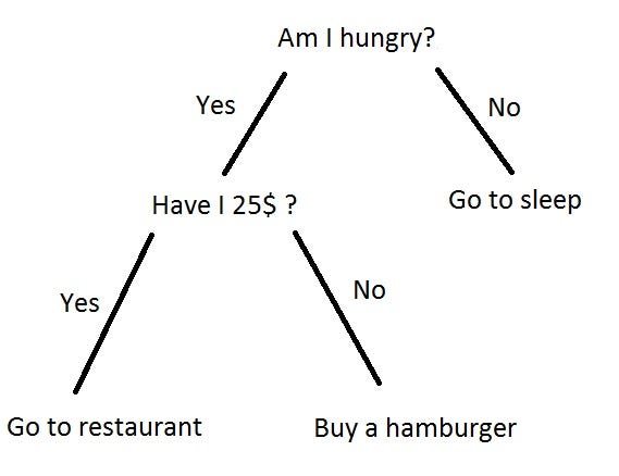
As is evident from the visualization, we are simply making a series of if-else decisions at each node of the tree and this leads us to one or more possible answers for the question that we are trying to find an answer to.
How do Decision Trees work?
Let us now try to understand the details of a decision tree algorithm in machine learning using a small dataset. We will use the iris dataset which is a very popular small dataset used in the machine learning and data science community for playing around with different concepts in these domains, including prediction. Here is the actual description of the iris dataset:
The iris data set gives the measurements in centimeters of the variables sepal length and width and petal length and width, respectively, for 50 flowers from each of 3 species of iris. The species are Iris setosa, versicolor, and virginica.
Here is a small snippet of how the data looks like:

Now suppose that given a set of sepal and petal widths and lengths for an iris flower, we want to identify which species of iris does that flower belongs to. This is a simple example of a machine learning task where given a set of input variables (Sepal.Length, Sepal.Width, Petal.Length and Petal.Width in our case), we are trying to predict an output variable (Species in our case). This is a good example of supervised learning and we will now see how we can use decision trees in order to perform this task.
To find a pattern in order to perform a good job of predicting the Species from the given sepal and petal measurements is a difficult task because we cannot simply look at one of the measurements at a time and decide the species to which the flower belongs to. We need to look at a combination of these measurements to finally pin down on the species to which the flower possibly belongs to. We will use the terms features to denote the input variables and the term class label to denote the output variable (Species). This is a classification scenario and we can call the model that we will build here as a classifier.
A naive approach to build our model would be to classify all the observations as the one with the highest frequency of Species in our data (in our case, the frequencies are the same as all the species have 50 observations). For instance, if we classify all the observations as versicolor, we get a prediction accuracy of 50/150 = 33.33% which is quite low but we should not underestimate the accuracy that can be obtained using this approach. The accuracy with this approach would depend on the distribution of our data and we might obtain an accuracy of 80% or even more. But this is a useless model and it completely ignores the features.
The decision-making process
Let us now see how a decision tree would handle this task. Let us recall and formulate that a decision tree is a nested sequence of if-else conditions based on the features and it will return a class label as an output at the end of each sequence. We can have a lot of decision trees and our task will be to find one that is good at our supervised learning problem.
Our decision tree would be made of several decision stumps which are the building blocks of a decision tree. Look at the image below to see what a decision stump would look like in our case:

Now our task is to find the best rule in terms of a threshold/label for each decision stump in our tree and we will do this by assigning a score to each possible decision stump that we look at and looking for the rule with the best score. What is one candidate for this score that immediately comes to our mind? Yes, you probably guessed it right. It’s the accuracy! We can calculate this by counting the number of observations that the model correctly classified. To consider this in relation to our problem, let us consider the rule from the image above which uses Petal.Width > 1.75 to decide the species of an example. Say that we obtain an accuracy a1 when we classify using this rule. Now, another similar rule might be Petal.Width > 2 and let’s say that we obtain an accuracy a2 using this rule. We simply select the first rule if a1 > a2 or select the second rule otherwise. There can be ties and they are usually broken randomly by the model. Similarly, we will have a lot of rules for all the other features and we need to use the best combination of such rules to obtain the maximum accuracy.
There is a whole can of worms in the process of how the model chooses its set of rules but what we need to understand is that the model will find the best rule by performing a search through a lot of possible candidates for that rule and deciding on the candidate that gives us the best score. For instance, the model can make rules based on
- Petal.Width > 0.00
- Petal.Width > 0.01
- Petal.Width > 0.02
- .
- .
- .
- Petal.Width > 10.00
The example provided above is just a glimpse of what actually happens and there are many candidate algorithms for carrying out this process. What we need to understand is that libraries like scikit-learn will perform this task optimally and provide us with the best rules by using algorithms that will speed up the rule search process.
Greedy nature of Decision Trees
It should be clear that decision stumps are a fairly simple class of models that use only 1 feature at a time and hence, not very accurate for most tasks. A decision tree, on the other hand, considers a lot of features and allows a sequence of split based on these features. It is important to note that they are a very general class of models and can attain high accuracies but the task of finding the optimal decision tree is not feasible computationally and therefore, we use what is called a greedy approach to choose our decision tree.
In this approach, we find the decision stump with the best rule and when the data gets split into two datasets using this rule, we recursively apply the same technique to the two obtained smaller datasets. What is important to learn and remember here is that we would not get the optimal decision tree using this process but what we obtain is a good decision tree to use for our prediction task. Another thing to note is that we can actually split the data such that any object gets completely split by itself and we would obtain each observation in a leaf node with the correct prediction. This would give us a 100% accuracy on our training dataset but this is something that is called overfitting and we would always want to avoid doing this. This is because such a model is not a generalized one and it won’t be able to predict well on new and unseen examples. For more information on overfitting, you can look at this blog post by William Koehrsen. Before we move on to implementing decision trees in python, let us look at some advantages and disadvantages in terms of only what we have learned so far.
Advantages
- Easy to understand - Decision trees and the underlying principle that they work on are easy to interpret and understand as compared to other complex machine learning algorithms.
- Fast to learn - Decision trees are relatively quite fast to learn as you will see when you learn about other complex algorithms.
Disadvantages
- Difficult to find an optimal set of rules - As we have already discussed, getting an optimal set of rules is hard and it is computationally inefficient to find such a set of rules and we have to use a greedy approach instead.
- Greedy splitting not accurate - This may require building very deep trees which might not be a good idea.
Implementing Decision Trees in Python
Now comes the most exciting part after having learned the theoretical stuff! We will implement a decision tree algorithm on the Iris dataset and make some predictions. We will then evaluate how our predictions performed using the accuracy obtained. Let’s get started without waiting any further. I bet you will be surprised with the amount of code that we will write for the whole process from getting the data to prediction!
# importing the iris dataset
from sklearn import datasets
from sklearn.model_selection import train_test_split

iris = datasets.load_iris()
X = iris.data
y = iris.target

X_train, X_test, y_train, y_test = train_test_split(
    X, y, test_size = 0.33, random_state = 42, shuffle = True)
The above code snippet will load the some required sklearn modules for us including the iris dataset itself. We then split the dataset into training and testing data with a 67-33% split using the train_test_split method from the model_selection module of sklearn library. Note that we need to shuffle the data before we split because we need our two datasets to be representative of the actual population (the shuffle argument takes care of this). Also, we use the random_state argument which will set a random seed for this split so that you get the exact same split as mine when you try to replicate this process on your machine.
# building our decision tree classifier and fitting the model
from sklearn import tree

model = tree.DecisionTreeClassifier()
model.fit(X_train, y_train)
In this code piece, we are importing the DecisionTreeClassifier class from sklearn which will be used to make our model. We then create an instance of that class which is used to fit the training data to the model.
# predicting on the train and the test data and assessing the accuracies
from sklearn.metrics import accuracy_score

pred_train = model.predict(X_train)
pred_test = model.predict(X_test)
train_accuracy = accuracy_score(y_train, pred_train)
test_accuracy = accuracy_score(y_test, pred_test)
print('Training accuracy is: {0}'.format(train_accuracy))
print('Testing accuracy is: {0}'.format(test_accuracy))
In the above code snippet, we are again importing a method to calculate our accuracy score in case of classification. We then use the predict method from tree in order to predict on our train and the test datasets. We then compare both the accuracies.
And that’s it! As I told you, you will be surprised by the amount of code that we would need to write a decision tree classifier using sklearn. I was definitely surprised when I first looked at this for the first time! These libraries make our lives much easier and we can actually concentrate on doing the machine learning instead of breaking our heads writing code to implement these algorithms from scratch, though it is definitely a good exercise in order to understand an algorithm from head to toe. I recommend doing that if you really want to learn the intricacies of a machine learning algorithm and the more you do that, the more you appreciate such libraries. Give it a try!
Analysis
When you run the last piece of code, you will see that we obtain an accuracy of 1.0 (100%) on both the training and the test data. This is because our data is relatively simple for the model to break down into patterns and it easily learns these patterns and classifies even the unseen data with a 100% accuracy. This is a good time to discuss the concept of depth in a decision tree. As we mentioned earlier, a decision tree can learn to perfectly fit the training data and it will require a large depth in order to achieve this. Depth is simply the maximum distance from the root to a leaf node in the tree. In order to see the effect of depth, let us try to train our model once again but with a maximum depth of 2 and see what happens.
# calculating the accuracy again with max_depth = 2

model2 = tree.DecisionTreeClassifier(max_depth = 2)
model2.fit(X_train, y_train)

pred_train = model2.predict(X_train)
pred_test = model2.predict(X_test)
train_accuracy = accuracy_score(y_train, pred_train)
test_accuracy = accuracy_score(y_test, pred_test)
print('Training accuracy with max_depth = 2 is: {0}'.format(train_accuracy))
print('Testing accuracy with max_depth = 2 is: {0}'.format(test_accuracy))
When you run this code, you will see a different result from what we obtained previously. If you set the random_state same as mine, you should get a training accuracy of 95% and a test accuracy of 98% which are once again, pretty good with such a small depth of the tree. Limiting the max depth results in a split where the leaf nodes may contain some examples from different categories which could have been further split to learn more accurate patterns. But again as I mentioned earlier, controlling the depth of the tree is an important factor if we don’t want to overfit our model on the training data. It is not clearly evident with the iris dataset but you can use some other dataset with this code and see what happens as you change the max_depth. In fact, tuning the hyperparameters is one of the most researched topics in machine learning and we are constantly trying to find new and novel ways to set their values (automatically) in order to obtain the best models.
Visualization
Let us look at the tree that we obtain after fitting our model to the data.
# visualizing our decision tree
# install graphviz using `pip install graphviz` or
# 'conda install graphviz' or `brew install graphviz`
import graphviz
from sklearn.tree import export_graphviz

dot_data = export_graphviz(model)
graphviz.Source(export_graphviz(model,
                                out_file=None,
                                feature_names=sorted(iris.feature_names),
                                class_names=["setosa", "versicolor", "virginica"],
                                impurity=False))
After you run this code, you can see a decision tree gets created which clearly states all the rules of splitting at each node. I’d suggest looking the nodes and their contents.
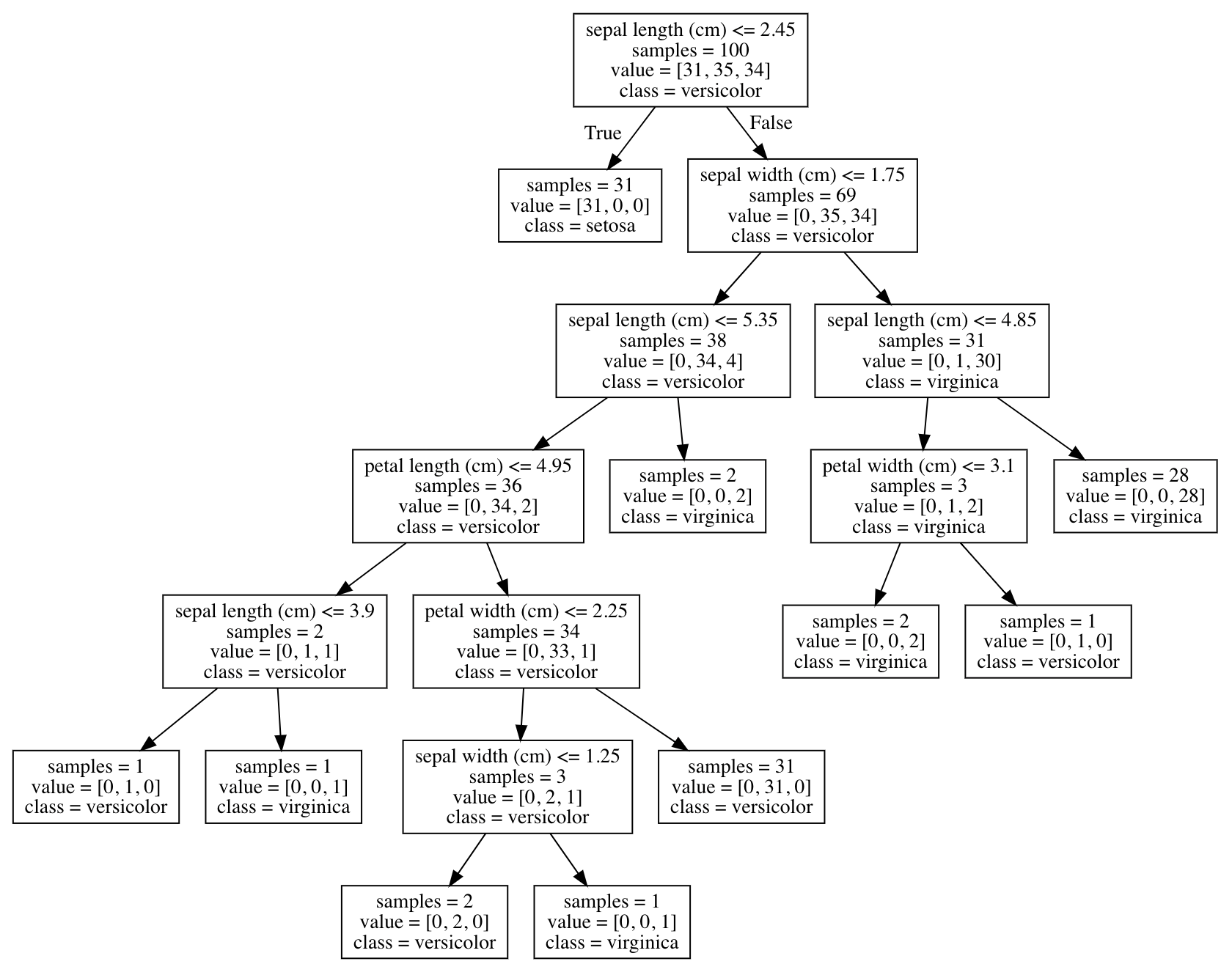
As you might have expected, the tree is a little big and complex and as they grow bigger, it becomes more difficult to directly comprehend them through human eyes. Let us visualize the second decision tree that we created (we can also export these trees to a pdf to zoom in on different parts and have a better look using the graphviz package).
# visualizing our decision tree with max_depth = 2
import graphviz
from sklearn.tree import export_graphviz

dot_data = export_graphviz(model2)
graphviz.Source(export_graphviz(model2,
                                out_file=None,
                                feature_names=sorted(iris.feature_names),
                                class_names=["setosa", "versicolor", "virginica"],
                                impurity=False))

As we discussed, the max depth in this tree is limited to 2 and we see a combination of different categories in the leaf nodes which could have been further split into more nodes to learn the pattern even better (which is what happens in the first case).
Conclusion
With this, we conclude the article and I hope this helped you understand the decision tree algorithm in a simple way. We also looked at the code using scikit-learn library in Python and I strongly suggest you play around with the code and new datasets to build and test your own decision trees. The full code for the tutorial can be found as a jupyter notebook on my github repository. We will learn about more interesting machine learning and deep learning algorithms in future posts!