
Building a Book Recommender System using Restricted Boltzmann Machines
Edit: Repository with complete code to run and test the system can be found here.
Motivation
I am an avid reader (at least I think I am!) and one of the questions that often bugs me when I am about to finish a book is “What to read next?”. It takes up a lot of time to research and find books similar to those I like. How cool would it be if an app can just recommend you books based on your reading taste? So why not transfer the burden of making this decision on the shoulders of a computer! This is exactly what we are going to do in this post.
We will try to create a book recommendation system in Python which can recommend books to a reader on the basis of the reading history of that particular reader. Once the model is created, it can be deployed as a web app which people can then actually use for getting recommendations based on their reading history. Let’s move forward with the task as we learn step by step how to create such a system in Python.
Note: This post is meant to be concise and to the point. We won’t be deviating from the relevant task to learn each and every involved concept in too much detail. In short, this post assumes some prior knowledge/intuition about Neural Networks and the ability to code in and understand Python. But I am sure even if you don’t have a prior experience with these things, you still get to take away a lot! So read on….

Architecture
There are a lot of ways in which recommender systems can be built. Some of them include techniques like Content-Based Filtering, Memory-Based Collaborative Filtering, Model-Based Collaborative Filtering, Deep Learning/Neural Network, etc. We will focus on learning to create a recommendation engine using Deep Learning. In particular, we will be using Restricted Boltzmann Machines (RBMs) as our algorithm for this task. The main reasons for that are:
- RBMs have the capability to learn latent factors/variables (variables that are not available directly but can be inferred from the available variables) from the input data.
- RBMs are unsupervised learning algorithms that have the capability to reconstruct input approximations from the data. They do this by trying to produce the probability distribution of the input data with a good approximation which helps in obtaining data points which did not previously exist in our data.
- They do this by learning a lower-dimensional representation of our data and later try to reconstruct the input using this representation.
Here is a representation of a simple Restricted Boltzmann Machine with one visible and one hidden layer:

For a more comprehensive dive into RBMs, I suggest you look at my blog post - Demystifying Restricted Boltzmann Machines.
The Network will be trained for 25 epochs (full training cycles) with a mini-batch size of 50 on the input data. The code is using tensorflow-gpu version 1.4.1 which is compatible with CUDA 8.0 (you need to use compatible versions of tensorflow-gpu and CUDA). You can check the version of TensorFlow compatible with the CUDA version installed on your machine here. You can also use the CPU-only version of TensorFlow if don’t have access to a GPU or if you are okay with the code running for a little more time. Let us summarize the requirements in bullet points below.
Requirements:
- Python 3.6 and above
- Tensorflow 1.4.1 (can be newer if a different CUDA version is Unsupervised)
- CUDA 8.0 (Optional - if you have access to a GPU)
- NumPy
- Pandas
- Matplotlib
Dataset
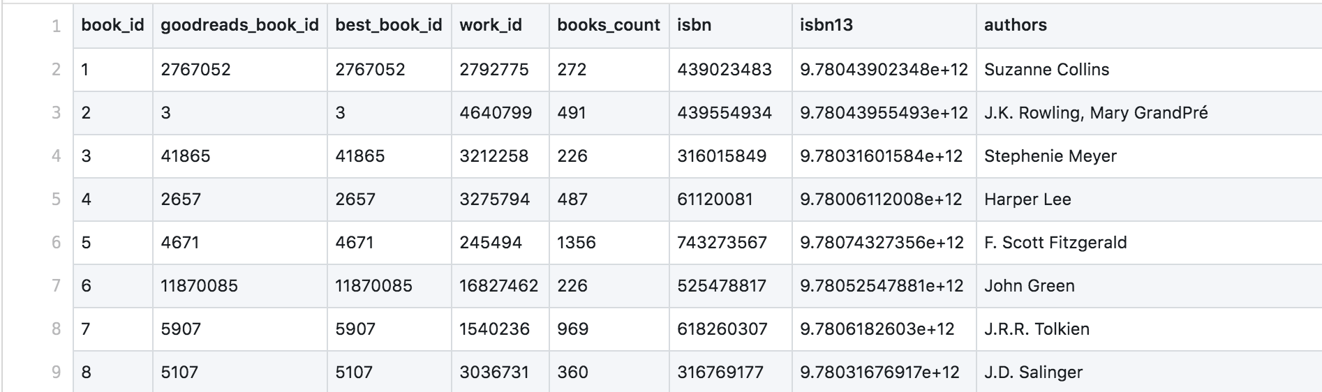
The required data was taken from the available goodbooks-10k dataset. The data comprises of 5 files in total (books, book_tags, ratings, to_read and tags). The file books.csv contains book (book_id) details like the name (original_title), names of the authors (authors) and other information about the books like the average rating, number of ratings, etc.
The file ratings.csv contains the mapping of various readers (user_id) to the books that they have read (book_id) along with the ratings (rating) given to those books by those users.

We also have the to_reads.csv file which gives us the mapping of the books (book_id) not yet read by different users (user_id) and this is quite helpful for our application as you will see later.

Data Preprocessing
The dataset is quite large and creates memory issues while allocating tensors with the total size of the available data, therefore we use a sample instead of the whole data. We will pick out a selected number of readers from the data (say ~ 200000) for our task. The data contains all but one of the variables important for the analysis. This missing variable is the Genre of the corresponding book. The Genre of the book could have been an important factor in determining the quality of the output from the application. Nevertheless, we will manually check the quality of recommendations for a random user later in the analysis. The data also doesn’t contain missing values in any of the variables relevant to our project. Let’s extract and modify the data in a way that is useful for our model.
We start by reading our data into variables.
ratings = pd.read_csv('data/ratings.csv')
to_read = pd.read_csv('data/to_read.csv')
books = pd.read_csv('data/books.csv')
Now, we will sort the ratings data according to user_id in order to extract the first 200000 users from the data frame. We do this because the dataset is too large and a tensor of size equal to the actual size of ratings data is too large to fit in our memory. You will need to play with this number in order to find an optimal number of rows that can fit inside your machine’s memory.
temp = ratings.sort_values(by=['user_id'], ascending=True)
ratings = temp.iloc[:200000, :]
The code below helps us to create an indexing variable which helps us uniquely identify each row after we group by user_id. Otherwise, we would not be able to perform the next task so easily which is to create the training data in a proper format that can be fed to our network later.
ratings = ratings.reset_index(drop=True)
ratings['List Index'] = ratings.index
readers_group = ratings.groupby("user_id")
After the above step, we need to create a list of lists as our training data where each list each list in the training data will be the ratings given to all the books by a particular user normalized into the interval [0,1] (or you can see it as the percentage score). All the books that the user has not read yet will be given the value 0. Also, note that the data needs to be normalized before it can be fed to a neural network and hence, we are dividing the ratings by 5. There are different ways to normalize the data and this is one of them.
total = []
for readerID, curReader in readers_group:
    temp = np.zeros(len(ratings))

    for num, book in curReader.iterrows():
        temp[book['List Index']] = book['rating'] / 5.0

    total.append(temp)

random.shuffle(total)
train = total[:1500]
valid = total[1500:]
Try not to print the training data as it would not be a good idea to print such a large dataset and your program may freeze (it probably will). We also divide the total data into training and validation sets which we will use later in order to decide on the optimal number of epochs for our training (which is important to avoid overfitting on the training data!).
hiddenUnits = 64
visibleUnits = len(ratings)

# Number of unique movies
vb = tf.placeholder(tf.float32, [visibleUnits])

# Number of features that we are going to learn
hb = tf.placeholder(tf.float32, [hiddenUnits])
W = tf.placeholder(tf.float32, [visibleUnits, hiddenUnits])  # Weight Matrix
In the above code chunk, we are setting our number of visible and hidden units. The choice of hidden units is random and there might be a really better value than this but is mostly as a power of 2 so as to optimally utilize matrix computations on GPU boards. The choice of visible units on the other hand, depends on the size of our input data. The weight matrix is created with the size of our visible and hidden units and you will see why this is the case and how this helps us soon!
A note on TensorFlow
We are using tf.placeholder here with the appropriate data type and size. It is like a literal placeholder which will be fed with a value always. We will feed values into it when we perform our training. It is the way tensorFlow was designed to work in the beginning.
TensorFlow uses a dataflow graph to represent your computation in terms of the dependencies between individual operations. This leads to a low-level programming model in which you first define the dataflow graph, then create a TensorFlow session to run parts of the graph across a set of local and remote devices. This required us to first design the dataflow graph of our model which we then run in a session (feeding appropriate values wherever required).
TensorFlow uses the tf.Session class to represent a connection between the client program—typically a Python program, although a similar interface is available in other languages—and the C++ runtime. A tf.Session object provides access to devices in the local machine, and remote devices using the distributed TensorFlow runtime. It also caches information about your tf.Graph (dataflow graph) so that you can efficiently run the same computation multiple times. What you need to know in simple terms is that the code is not actually executing unless we run the session (it is where all the stuff happens).
TensorFlow has evolved a lot over the 3 years from the time when it was created/released and this dataflow graph implementation is typically not used in the beginning these days when starting to learn tensorFlow. Some really good and easy to implement high-level APIs like Keras are now used to learn and starting to write code in tensorFlow (tf.keras is the tensorFlow implementation of the API).
For more information on graphs and sessions, visit the tensorFlow official documentation page. I will keep the detailed tutorial and implementation details in tensorFlow for another blog post. Let us move on with our code and understand what is happening rather than focusing on tensorFlow syntax.
v0 = tf.placeholder("float", [None, visibleUnits])
_h0 = tf.nn.sigmoid(tf.matmul(v0, W) + hb)  # Visible layer activation
# Gibb's Sampling
h0 = tf.nn.relu(tf.sign(_h0 - tf.random_uniform(tf.shape(_h0))))
So in the above piece of code, we are now doing something similar to one forward pass of a feed forward neural network and obtaining our output for the hidden layer (remember we have no output layer in this network). This is our input processing phase and is the beginning of Gibbs Sampling. Note that we are using a Rectified Linear Unit as our activation function here. Other activation functions such as the sigmoid function and the hyperbolic tangent function could also be used but we use ReLU because it is computationally less expensive to compute than the others. This is only one of the reasons why we use them. For more information on what these activation functions are, look at my blog post Neural Networks - Explained, Demystified and Simplified and for a more clear understanding of why ReLUs are better look at this great answer on StackExchange. Let’s move on!
# Hidden layer activation
_v1 = tf.nn.sigmoid(tf.matmul(h0, tf.transpose(W)) + vb)
v1 = tf.nn.relu(tf.sign(_v1 - tf.random_uniform(tf.shape(_v1))))
h1 = tf.nn.sigmoid(tf.matmul(v1, W) + hb)
This is the Reconstruction phase and we recreate the input from the hidden layer activations.
# Learning rate
alpha = 0.6

# Creating the gradients
w_pos_grad = tf.matmul(tf.transpose(v0), h0)
w_neg_grad = tf.matmul(tf.transpose(v1), h1)
Setting the learning rate and creating the positive and the negative gradients using matrix multiplication which will then be used in approximating the gradient of an objective function called Contrastive Divergence (find more information on this here).
# Calculate the Contrastive Divergence to maximize
CD = (w_pos_grad - w_neg_grad) / tf.to_float(tf.shape(v0)[0])

# Create methods to update the weights and biases
update_w = W + alpha * CD
update_vb = vb + alpha * tf.reduce_mean(v0 - v1, 0)
update_hb = hb + alpha * tf.reduce_mean(h0 - h1, 0)
The above code is what updates our weight matrix and the biases using the Contrastive divergence algorithm which is one of the common training algorithms for RBMs. All such common algorithms approximate the log-likelihood gradient given some data and perform gradient ascent on these approximations.
# Set the error function, here we use Mean Absolute Error Function
err = v0 - v1
err_sum = tf.reduce_mean(err * err)
This code snippet simply sets the error function for measuring the loss while training on the data and will give us an idea of how well our model is creating the reconstructions of the input data.
# Current weight
cur_w = np.random.normal(loc=0, scale=0.01, size=[visibleUnits, hiddenUnits])

# Current visible unit biases
cur_vb = np.zeros([visibleUnits], np.float32)

# Current hidden unit biases
cur_hb = np.zeros([hiddenUnits], np.float32)

# Previous weight
prv_w = np.zeros([visibleUnits, hiddenUnits], np.float32)

# Previous visible unit biases
prv_vb = np.zeros([visibleUnits], np.float32)

# Previous hidden unit biases
prv_hb = np.zeros([hiddenUnits], np.float32)
The above code created weights and bias matrices for computation in each iteration of training and initialized them with appropriate values and data types (data types are important in numpy, set them appropriately or you will face unwanted errors while running your code if the types are incompatible). The weights are initialized with random values from a standard normal distribution with a small standard deviation. For a highly comprehensive guide more information on setting up and initializing various parameters and variables, look at this awesome guide by Geoffrey Hinton on training RBMs.
# Running the session
config = tf.ConfigProto()
config.gpu_options.allow_growth = True
sess = tf.Session(config=config)
sess.run(tf.global_variables_initializer())
Now we initialized the session in tensorFlow with appropriate configuration for using the GPU effectively. You may need to play around with these settings a little bit of you are trying to use a GPU for running this code.
def free_energy(v_sample, W, vb, hb):
    ''' Function to compute the free energy '''
    wx_b = np.dot(v_sample, W) + hb
    vbias_term = np.dot(v_sample, vb)
    hidden_term = np.sum(np.log(1 + np.exp(wx_b)), axis = 1)
    return -hidden_term - vbias_term
Boltzmann Machines (and RBMs) are Energy-based models and a joint configuration, \((\textbf{v}, \textbf{h})\) of the visible and hidden units has an energy given by:
\[\displaystyle E(\textbf{v}, \textbf{h}) = − \sum_{i∈visible} a_i v_i − \sum_{j∈hidden} b_jh_j − \sum_{i,j} v_ih_jw_{ij}\]where \(v_i\), \(h_j\) are the binary states of visible unit \(i\) and hidden unit \(j\), \(a_i\), \(b_j\) are their biases and \(w_{ij}\) is the weight between them.
We create this function to calculate the free energy of the RBM using the vectorized form of the above equation. To know how to compute the free energy of a Restricted Boltzmann Machine, I suggest you to look at this great discussion on StackExchange. Now we move on to the actual training of our model.
epochs = 60
batchsize = 100
errors = []
energy_train = []
energy_valid = []
for i in range(epochs):
    for start, end in zip(range(0, len(train), batchsize), range(batchsize, len(train), batchsize)):
        batch = train[start:end]
        cur_w = sess.run(update_w, feed_dict={
                         v0: batch, W: prv_w, vb: prv_vb, hb: prv_hb})
        cur_vb = sess.run(update_vb, feed_dict={
                          v0: batch, W: prv_w, vb: prv_vb, hb: prv_hb})
        cur_hb = sess.run(update_hb, feed_dict={
                          v0: batch, W: prv_w, vb: prv_vb, hb: prv_hb})
        prv_w = cur_w
        prv_vb = cur_vb
        prv_hb = cur_hb

    energy_train.append(np.mean(free_energy(train, cur_w, cur_vb, cur_hb)))
    energy_valid.append(np.mean(free_energy(valid, cur_w, cur_vb, cur_hb)))

    errors.append(sess.run(err_sum, feed_dict={
                  v0: train, W: cur_w, vb: cur_vb, hb: cur_hb}))
    if i % 10 == 0:
        print("Error in epoch {0} is: {1}".format(i, errors[i]))
This code trains our model with the given parameters and data. Note that we are now feeding appropriate values into the placeholders that we created earlier. Each iteration maintains previous weights and biases and updates them with the value of current weights and biases. Finally, error is appended after each epoch to a list of errors which we will use to plot a graph for the error.
fig, ax = plt.subplots()
ax.plot(energy_train, label='train')
ax.plot(energy_valid, label='valid')
leg = ax.legend()
plt.xlabel("Epoch")
plt.ylabel("Free Energy")
plt.savefig("free_energy.png")
plt.show()
Also note that we are calculating the free energies using our training and validation data. The plot shows the average free energy for training and the validation dataset with epochs.

If the model is not overfitting at all, the average free energy should be about the same on training and validation data. As the model starts to overfit the average free energy of the validation data will rise relative to the average free energy of the training data and this gap represents the amount of overfitting. So we can determine the number of epochs to run the training for using this approach. Looking at the plot, we can safely decide the number of epochs to be around 50 (I trained the model with 60 epochs after looking at this plot). Geoffrey Hinton summarizes the best practices for selecting the hyperparameters quite well here and this is one of his suggestions to arrive at a good number of epochs.
plt.plot(errors)
plt.xlabel("Epoch")
plt.ylabel("Error")
plt.savefig("error.png")
plt.show()
After we are done training our model, we will plot our error curve to look at how the error reduces with each epoch. As mentioned, I trained the model for 60 epochs and this is the graph that I obtained.

Now that we are done with training our model, let us move on to the actual task of using our data to predict ratings for books not yet read by a user and provide recommendations based on the reconstructed probability distribution.
user = 22
inputUser = [train[user]]
Here we are specifying a random reader from our data. We will use this reader in our system to provide book recommendations (feel free to choose any user existing in the data).
# Feeding in the User and Reconstructing the input
hh0 = tf.nn.sigmoid(tf.matmul(v0, W) + hb)
vv1 = tf.nn.sigmoid(tf.matmul(hh0, tf.transpose(W)) + vb)
feed = sess.run(hh0, feed_dict={v0: inputUser, W: prv_w, hb: prv_hb})
rec = sess.run(vv1, feed_dict={hh0: feed, W: prv_w, vb: prv_vb})
The above code passes the input from this reader and uses the learned weights and bias matrices to produce an output. This output is the reconstruction of ratings by this user and this will give us the ratings for the books that the user has not already read.
# Creating recommendation score for books in our data
ratings["Recommendation Score"] = rec[0]

# Find the mock user's user_id from the data
cur_user_id = ratings.iloc[user]['user_id']

# Find all books the mock user has read before
read_books = ratings[ratings['user_id'] == cur_user_id]['book_id']

# converting the pandas series object into a list
read_books_id = read_books.tolist()

# getting the book names and authors for the books already read by the user
read_books_names = []
read_books_authors = []
for book in read_books_id:
    read_books_names.append(
        books[books['book_id'] == book]['original_title'].tolist()[0])
    read_books_authors.append(
        books[books['book_id'] == book]['authors'].tolist()[0])
We now created a column for predicted recommendations in our ratings data frame and then find the books that the user has already read. We also obtain the book title and author information for these books. This is what the information looks like:

# Find all books the mock user has 'not' read before using the to_read data
unread_books = to_read[to_read['user_id'] == cur_user_id]['book_id']
unread_books_id = unread_books.tolist()

# extract the ratings of all the unread books from ratings dataframe
unread_with_score = ratings[ratings['book_id'].isin(unread_books_id)]

# grouping the unread data on book id and taking the mean of the recommendation scores for each book_id
grouped_unread = unread_with_score.groupby('book_id', as_index=False)[
    'Recommendation Score'].mean()
Now using the above code, we find the book not already read by this user (we use the third file to_read.csv for this purpose). We also find the ratings for these books and summarize them to their means. We are doing this because we will get a rating each time this book is encountered in the dataset (read by another user).
# getting the names and authors of the unread books
unread_books_names = []
unread_books_authors = []
unread_books_scores = []
for book in grouped_unread['book_id']:
    unread_books_names.append(
        books[books['book_id'] == book]['original_title'].tolist()[0])
    unread_books_authors.append(
        books[books['book_id'] == book]['authors'].tolist()[0])
    unread_books_scores.append(
        grouped_unread[grouped_unread['book_id'] == book]['Recommendation Score'].tolist()[0])
Now that we obtained the ratings for the unread books, we next extracted the titles and author information so that we can see what books got recommended to this user by our model. This is what we see:

# creating a data frame for unread books with their names, authors and recommendation scores
unread_books_with_scores = pd.DataFrame({
    'book_name': unread_books_names,
    'book_authors': unread_books_authors,
    'score': unread_books_scores
})

# creating a data frame for read books with the names and authors
read_books_with_names = pd.DataFrame({
    'book_name': read_books_names,
    'book_authors': read_books_authors
})

# sort the result in descending order of the recommendation score
sorted_result = unread_books_with_scores.sort_values(
    by='score', ascending=False)

# exporting the read and unread books  with scores to csv files
read_books_with_names.to_csv('results/read_books_with_names.csv')
sorted_result.to_csv('results/unread_books_with_scores.csv')
print('The books read by the user are:')
print(read_books_with_names)
print('The books recommended to the user are:')
print(sorted_result)
In this last step, we are simply creating relevant data frames for read and unread books by this user to export the results to a .csv file and printing it to console.
Results
Now that we are done with all our code for the book recommender system, I want you to look carefully at the books read by the user and the books recommended to the user. Do you notice any similarity? I couldn’t figure it out on my own (guess I am not an avid reader at all!). If even you can’t figure out by yourself, let me tell you. The top 2 books recommended to this user are romance novels and guess what? The books already read by this user consisted of 17% romantic novels! The list shown for the already read books is not complete and there are a lot more that this user has read. Though there is always a scope for improvement, I’d say with confidence that the system performed really well and that some really good books can be recommended for users using this system.

Conclusion
With that, I conclude this post and encourage you all to build awesome recommender systems with not only books but different categories of data. Recommendation systems are a core part of business for organizations like Netflix, Amazon, Google, etc. and other tech giants. Building robust recommender systems leading to high user satisfaction is one of the most important goals to keep in mind when building recommender systems in production. But there are a lot of challenges when we work at such a large scale:
- Dynamic prediction – Precomputing all the recommendations is almost impossible and very inefficient when we are working at such a large scale with so many users.
- Optimizing response time – Dynamic predictions will require reducing the query and response times to be minimum so that the user can be provided with the results quickly.
- Frequency of updates – As more and more new data gets accumulated, it is important to frequently update the model to incorporate this information.
- Prediction on unseen data – We will require to deal with unseen users and continuously changing features.
We will probably talk about how to handle recommender systems at large scale in a future post! All the code for this tutorial is available on my GitHub repository.
Note: I will optimize/update the code to use numpy and other libraries and make it object oriented. Feel free to add any suggestions and questions in the comments section below!