
All you need to know about Gradient Descent
Introduction
Most deep learning algorithms (also machine learning algorithms, in general) involve optimization of some sort which refers to the task of minimizing or maximizing a function \(f(x)\) by changing the values of the input \(x\). The convention is to minimize the function and if we need to maximize it in some scenario (for example a transformation of the function), we will minimize \(-f(x)\) instead of maximizing \(f(x)\). This keeps things less confusing and consistent.
The function that we want to minimize is often called the objective function. It is also called by other names such as cost function, loss function, error function, etc. This is the function which we define using the problem that we want to solve using deep learning and an appropriate choice of properties that make the function easier to deal with for the optimization task. The convention used for defining the value that minimizes or maximizes the function is denote by \(x^* =\) arg min\(f(x)\). Our goal is to find this optimal value (or a similar value not so optimal in some cases) that minimizes our objective function.
Let us now review some basic calculus that we need to know in order to understand how gradient descent works.
Calculus basics
For a function \(y = f(x)\), we define its derivative at a point \(x\) as the slope of the function \(x\). The slope gives us an idea of the scale of change we see in the value of the function (\(y\)) if we change the value of \(x\) infinitesimally. This is denoted by \(f'(x)\) or \(\frac{dy}{dx}\). Suppose we change the value of \(x\) by an infinitesimally small value \(\epsilon\). Then using the derivative of the function we can write:
\[\frac{dy}{dx} = f'(x) = \frac{f(x + \epsilon) - f(x)}{\epsilon}\]This can be used to get the approximate value of the function at the point \(x + \epsilon\) which will be given by:
\[f(x + \epsilon) \approx f(x) + \epsilon f'(x)\]The way this derivative is useful for us is that it tells us how to change \(x\) in order to get a small improvement in \(y\).
Now we know that the derivative of a function at a point gives us the slope of the function. When we have a zero slope at a point \(x\) (i.e., \(f'(x) = 0\)), we call \(x\) as a critical point or a stationary point. This stationary point can either be a local minimum or a local maximum or none of the above two. When the value of \(f(x)\) is lower than its value at of all the neighbors of \(x\), then \(x\) is called the local minimum. Similarly, if the value of \(f(x)\) is greater than its value at all the neighboring points of \(x\), then \(x\) is called the local maximum. There are functions where the value of \(f(x)\) is greater than some of \(x\)’s neighbors and less than some other neighbors. Such a point is neither a minimum nor a maximum and is known as a saddle point. Let us visualize these critical points in 1-D. Contrast the saddle point as compared to the local minimum and the local maximum point.

Using the concept of the derivative above, we can see that the value of the function \(f(x)\) at \(x - \epsilon * sign(f'(x))\) always takes \(f(x)\) towards a lower value. This process of using the gradient (derivative) of \(f(x)\) to reach a point where the value of the function is minimum is known as gradient descent. We are simply moving \(f(x)\) to a lower value by moving \(x\) in a direction opposite to the sign of the derivative of \(f(x)\) in small steps defined by \(\epsilon\). Take a moment and think about it. Look at the image below and convince yourselves that the above proposition holds true.

Here is a better illustration of how gradient descent is used to reach a local minima using the method described above from the Deep Learning book by Goodfellow et al. (I highly recommend this book for someone who wants to go deep into the working of modern deep learning practices).

Now that we know what a local minima or a local maxima is, let us talk about the global minima and maxima. In general, we will ignore talking about maxima from now on as we will align our discussion with the convention that we need to minimize the objective function. A global minima is the point where the function’s value is the minimum of all the possible points in the domain of the function. In other words, there is no other point \(x\) such that \(f(x) < f(x^*)\) where \(x^*\) is the global minima of the function \(f(x)\). Notice the strict inequality there. This means that there can be multiple points which can act as the global minima. It should be clear that there can also be local minima which are not globally optimal.
A challenge which is very common in the context of deep learning is that objective functions often are not so simple and we may have a lot of local minima and a lot of saddle points which makes it difficult to find the global optimum. Also, the functions are mostly multidimensional which makes it even more tricky to arrive at the global optimal value. Due to all of this, we often settle for a value of \(f\) which is very low, but not necessarily the most optimal value and as you will see when you further study deep learning, this method of arriving at a low value of the objective function finds this value quickly enough to be useful. To understand this, look at the picture below.

Optimization in multiple dimensions
We often minimize functions that have multiple inputs: \(f: \mathbb{R}^{n} \rightarrow \mathbb{R}\). This will need us to obtain a single scalar value for the concept of minimization to make sense. Most real world problems are not that simple and are mostly multi-dimensional and so let us try to understand how gradient descent is used in multiple dimensions. Suppose instead of a single number, now the input is a vector \(\boldsymbol{x}\) in \(n\) dimensions. So \(\boldsymbol{x} = \{x_1, x_2, x_3, .... , x_n\}\).
Now, to incorporate the effect of each component of the input vector, we will use the concept of partial derivatives. Partial derivatives are similar to the normal derivatives that we saw above with the only difference being that they capture the gradient of the function in a specific direction defined by that specific component. For instance, if the input is a 2-D vector then one of its partial derivatives would be the gradient in the x-direction and the other in the y-direction. Partial derivatives are denoted by a different symbol (\(\delta\) instead of \(d\)) and the partial derivative of a function \(y = f(\boldsymbol{x})\) with respect to \(x_i\) would be written as \(\frac{\delta y}{\delta x_i}\). So the gradient of \(f\) will be the vector of partial derivatives of \(f\) with respect to all the components \(x_i\) of the input vector \(\boldsymbol{x}\) and it is denoted by \(\nabla_{\boldsymbol{x}} f(\boldsymbol{x})\). The critical points in multiple dimensions are the points where the partial derivatives with the respect to all the components is zero (i.e., every element of the gradient is zero).
In more mathematical terms, the directional derivative of the function in the direction \(\boldsymbol{u}\) is the slope of the function in the directional derivative defined by \(u\) (where \(u\) is a unit vector). In other words, the directional derivative of the function \(f(x + \alpha\boldsymbol{u})\) with respect to \(\alpha\), evaluated at \(\alpha = 0\). The derivative of \(f(x + \alpha\boldsymbol{u})\) with respect to \(\alpha\) would be given by
\[\frac{\delta}{\delta \alpha} f(x + \alpha\boldsymbol{u})\] \[= \boldsymbol{u}f'(x + \alpha\boldsymbol{u}) \mid_{\alpha = 0}\]\(\hspace{7cm} = \boldsymbol{u}^\top \nabla_{\boldsymbol{x}} f(\boldsymbol{x}) \hspace{1cm}\) (when \(\alpha = 0\))
We will need to find the direction in which \(f\) decreases the fastest in order to minimize it (reach the global or a good local minimum). To do that, we can use the directional derivative. We need to solve for a \(u\) such that:
\[= \underset{\boldsymbol{u}, \boldsymbol{u^\top}\boldsymbol{u} = 1} {\text{min}} \boldsymbol{u}^\top \nabla_{\boldsymbol{x}} f(\boldsymbol{x})\] \[\underset{\boldsymbol{u}, \boldsymbol{u^\top}\boldsymbol{u} = 1} {\text{min}} \mid\mid\boldsymbol{u}\mid\mid_2 \mid\mid\nabla_{\boldsymbol{x}} f(\boldsymbol{x})\mid\mid_2 \text{cos} \ \theta\]and after substituting \(\mid\mid\boldsymbol{u}\mid\mid_2 = 1\) and ignoring the second factor as it doesn’t depend on \(\boldsymbol{u}\), we arrive at \(\text{min}_u \ \text{cos}\ \theta\). We will get the minimum of this quantity when \(\theta = 180\) degrees which means that the gradient and \(\boldsymbol{u}\) are in the exact opposite directions. This means that if the gradient is in the direction of uphill, the function will move towards the minimum when we move directly opposite to the gradient (direction of downhill). This is known as the method of steepest descent or gradient descent. This helps us propose a new point at every step which is given by \((x - \epsilon \nabla_{\boldsymbol{x}} f(\boldsymbol{x}))\) where \(\epsilon\) is a small positive scalar called the learning rate (which I am sure you might have heard about if you have read about neural networks or deep learning algorithms in general). This number is chosen such that the the value of the function at this new point will be smaller than the previous value. Typically, it is initialized as a small constant as if it is too large, we might end up in a region of the function which does not converges to the minimum and starts diverging instead. There are various methods and empirical techniques that have been used to arrive at a good learning rate. Look at this article if you want to read about some techniques to select a good learning rate for your project. Sometimes, we just try out different values of \(\epsilon\) and choose the one which minimizes our objective function the most and this strategy is known as line search. The criteria for the method of gradient descent to converge is that all the partial derivatives become zero at a point (every element of the gradient becomes zero). This might not always happen and we need to be satisfied with a small enough difference between the gradient and zero defined by a tolerance value while some other times, it is possible to directly solve for the value where the gradient becomes zero (\(\nabla_{\boldsymbol{x}} f(\boldsymbol{x}) = 0\)). Here is a picture depicting how different starting points can lead to different local optima when found using gradient descent:
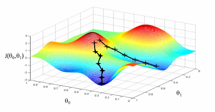
One important thing to note is that the convergence point of gradient descent depends on the initialization of the parameters. Gradient descent is not limited to continuous spaces and can be optimized to discrete spaces. Sometimes it is also possible to have both the input and the output as vectors and in those cases, we need to deal with the above method using Jacobian and Hessian matrices but we are not going to go into that. You can read more about the it from page 84 of this chapter from the Deep Learning Book.
Now we will talk about the most used algorithm in the field of deep learning based on gradient descent called Stochastic Gradient Descent.
Stochastic Gradient Descent
Stochastic Gradient Descent or SGD is the most commonly used algorithm in deep learning for the task of optimizing the objective function. Before looking at what the algorithm is, let us try to understand the problem with basic gradient descent which this algorithm addresses. The cost function used in statistical estimation and machine learning usually involves a sum of all the training examples over a per-example loss function. For instance:
\[Q(w) = \frac{1}{m} \displaystyle \sum_{i=1}^{m} Q_i(w)\]where we are trying to estimate the parameter \(w\) which minimizes the objective function \(Q(w)\). Each \(Q_{i}\) is typically associated with the \(i\)-th observation in the data set (used for training). To get the gradient of these additive cost functions, we require a sum over all the training examples:
\[\nabla_{\boldsymbol{\theta}} Q(\boldsymbol{\theta}) = \frac{1}{m} \displaystyle \sum_{i=1}^{m} \nabla_{\boldsymbol{\theta}}Q(\boldsymbol{x}^{(i)}, y^{(i)}, \boldsymbol{\theta })\]where \(\boldsymbol{\theta}\) is nothing but the weight matrix that we are trying to find an optimal value for. Most of the times in deep learning, we find ourselves minimizing the gradient of the negative log-likelihood of a function or of a least squares sum. The important thing to note here is that this will require us to sum over all the \(m\) training examples and this task becomes computationally intensive and takes up more and more time (\(O(m)\) in time) as the number of examples in our training set increases. In machine learning, since large training sets are good for generalization, they also make the task more computational expensive.
In order to tackle this, we use a stochastic approximation of the gradient descent optimization. It is called stochastic because samples are selected randomly (or shuffled) instead of as a single group (as in standard gradient descent) or in the order they appear in the training set. In this algorithm, instead of using the whole training dataset with \(m\) examples for the update of weights using the method described in gradient descent, we use a small subset of the training examples (typically between 10 to 1000 examples). This makes the cost per update of SGD independent of the number of training examples. The estimate of the gradient is now calculated using a subset of the training set with \(m'\) examples which now becomes:
\[\boldsymbol{g} = \frac{1}{m'} \displaystyle \sum_{i=1}^{m'} \nabla_{\boldsymbol{\theta}}Q(\boldsymbol{x}^{(i)}, y^{(i)}, \boldsymbol{\theta })\]using the examples from the mini-batch \(\mathbb{B}\). The estimate of \(\boldsymbol{\theta}\) will now follow the path downhill with
\[\boldsymbol{\theta} \leftarrow \boldsymbol{\theta} - \epsilon \boldsymbol{g}\]where \(\epsilon\) is the learning rate. One difference to note here is the way the term Stochastic Gradient Descent is being used here. To be specific, SGD is the stochastic approximation of gradient descent which uses only a single example per iteration. This is the extreme case of what we actually use in practice which we described above and it is called mini-batch stochastic gradient descent. So mini-batch stochastic gradient descent is a compromise between full-batch gradient descent and SGD. Now that we have an idea of what gradient descent is and of the actual variation that is used in practice (mini-batch SGD), let us learn how to implement these algorithms in python.
Implementation
Our learning doesn’t stop at just the theory of these concepts as we would want to implement and use these algorithms in our projects and what not! In my opinion, learning the theory of a concept and actually implementing it in code has a lot of difference. This difference is evident when you see either the code implementation or the theory in isolation but when you see both of these together (jumping back and forth between the code and the theory until you understand it fully), you learn the concept more effectively and efficiently and are more confident with it.
I like to see the learning of any machine learning concept using code and theory modeled as Kullback-Leibler Divergence. If we have two separate probability distributions \(P(x)\) and \(Q(x)\) over the same random variable \(x\), we can measure how different these two distributions are using the Kullback-Leibler (KL) divergence. I like to see the theory and code part as these two probability distributions and the process of jumping back and forth between the code and theory modeled as Gibbs Sampling. As we make more iterations jumping back and forth, the KL divergence goes towards zero and that is the state we want us to be in!
Okay, stepping out of the analogy now (forgive me, I can’t stop myself from creating analogies between the real word and the deep learning world!), we will be implementing both full-batch gradient descent and mini-batch SGD using python (both base Numpy and TensorFlow versions).
Gradient Descent in Python
In order to understand the full implementation and use of gradient descent in a problem and not just look at the raw code for the algorithm, let us apply gradient descent in a linear regression problem and see how it can be used to optimize the objective function (least squares estimate in this case).
Linear Regression with Gradient Descent
# importing required libraries (numpy only in this case)
import numpy as np

# creating a random dataset with some relation
np.random.seed(1245)
X = np.linspace(1, 10, 100)[:, np.newaxis]
y = np.sin(X) + 0.1 * np.power(X, 2) + 0.5 * np.random.randn(100, 1)

# normalizing X to keep the algorithm numerically stable
X = X / np.max(X)

# randomly dividing the data into train and test sets (70-30 split)
perm = np.random.permutation(len(X))
div = 70

train_X = X[perm[: div]]
train_y = y[perm[: div]]
test_X = X[perm[div:]]
test_y = y[perm[div:]]
The above code snippet contains the code to get started with our regression problem. We are creating a dataset with some relation between the response (\(y\)) and the predictor variables (\(X\)). Note that of you run this code in a Jupyter Notebook, you will need to add the random seed in every cell where there is some randomness in generating the data or the variables (it is just the way how things are for now, sadly!). Now we will write a function which will return the gradient for us that we will use to update our parameters step by step.
# function to get the gradient and the means squared error
def gradient(x, y, w, b):
    y_pred = x.dot(w).flatten() + b
    error = y.flatten() - y_pred
    mse = (1.0/len(x)) * np.sum(np.power(error, 2))
    grad_w = -(2.0/len(x)) * error.dot(x)
    grad_b = -(2.0/len(x)) * np.mean(error)
    return grad_w, grad_b, mse
The above code implements gradient descent to reach the minimum for a linear regression problem. Note that linear regression can be optimized without optimizing techniques like gradient descent because we are able to convert the problem into a nicer closed form equation format which from where we can directly obtain the solution that will result in the least squares fit. We nevertheless, use gradient descent here in order to understand the implementation in python.
The equations that we see above are obtained when we apply the partial differentiation to the equation of the loss function which in this case is just the sum of the errors squared:
\[Q(x, y, w) = \frac{1}{m} \displaystyle \sum_{i=1}^m(w_0 + w_1 x_i - y_i)^2\]We now take the partial derivatives of the objective function with respect to both the intercept (or the bias term, \(w_0\)) and the slope (or the weight, \(w_1\)) in order to obtain the partial gradients with respect to these parameters.
\[\frac{\delta}{\delta w_1} Q(x, y, w) = \frac{-2}{m} \displaystyle \sum_{i=1}^m(w_0 + w_1 x_i - y_i) * x_i\] \[\frac{\delta}{\delta w_0} Q(x, y, w) = \frac{-2}{m} \displaystyle \sum_{i=1}^m(w_0 + w_1 x_i - y_i)\]I am not using the matrix notation here in which case, we will need to take transpose of appropriate matrices in order to multiply them properly. Convince yourselves that these equations are what you see in the code for the gradient function implemented above (the code is using matrix algebra!). Now we initialize the variables and parameters and run our algorithm until convergence which is defined by a tolerance value for the slope parameter (\(w_1\)).
# initializing variables
w = np.random.randn(1)
b = np.random.randn(1)
alpha = 0.4
tol = 1e-5

iteration = 1

# running the algorithm until convergence
while True:
    grad_w, grad_b, err = gradient(train_X, train_y, w, b)

    #update the weights
    w_curr =  - alpha * grad_w
    b_curr = - alpha * grad_b
    #stopping condition
    if np.sum(w - w_curr) < tol:
        print("The algorithm converged!")
        break

    if iteration % 100 == 0:
        print("Iteration: {0}, Error: {1}".format(iteration, err))

    iteration += 1
    w = w_curr

print("w = {0}".format(w))
print("Test Cost = {0}".format(gradient(test_X, test_y, w, b)[2]))
The output of the above code when run is:
The algorithm converged!
w = [0.83129165]
b = [-0.37241604]
Test Cost = 16.010686284045498
which gives us the obtained weights and biases that optimizes the objective function. The procedure is the same whether you use gradient descent in linear regression or for neural networks. Now, let us see how libraries like TensorFlow make our lives easier by implementing these optimization functions efficiently in their codebase.
Gradient Descent using TensorFlow
We will use the same dataset for this implementation and without wasting any mental energy further, let’s jump into the code straight on!
import numpy as np
import tensorflow as tf

np.random.seed(1245)
X = np.linspace(1, 10, 100)[:, np.newaxis]
Y = np.sin(X) + 0.1 * np.power(X, 2) + 0.5 * np.random.randn(100, 1)

# normalizing X to keep the algorithm numerically stable
X = X / np.max(X)

perm = np.random.permutation(len(X))
div = 70

train_X = X[perm[: div]]
train_y = Y[perm[: div]]
test_X = X[perm[div:]]
test_y = Y[perm[div:]]
The above code is common for the previous implementation. Now we will write a function to return the predictions and the mean squared error.
def calc(x, y, w, b):
    # Returns predictions and error
    predictions = tf.multiply(x, w) + b
    error = tf.reduce_mean(tf.square(y - predictions))
    return [ predictions, error ]
# x and y are placeholders for our training data
x = tf.placeholder("float64")
y = tf.placeholder("float64")

w = tf.Variable(np.random.randn(1), name = "w")
b = tf.Variable(np.random.randn(1), name = "b")

# Our model of y = a*x + b
y_model = tf.multiply(x, w) + b

# Our error is defined as the square of the differences
error = tf.square(y - y_model)

# The Gradient Descent Optimizer with a optimized implementation of gradient descent
train_op = tf.train.GradientDescentOptimizer(0.4).minimize(error)

# Normal TensorFlow - initialize values, create a session and run the model
model = tf.global_variables_initializer()
The above code initializes the required variables using TensorFlow and creates the computational graph that we will later execute in a tf.Session().
with tf.Session() as session:
    session.run(model)
    for i in range(70):
        x_value = train_X[i]
        y_value = train_y[i]
        session.run(train_op, feed_dict={x: x_value, y: y_value})

    w_value = session.run(w)
    b_value = session.run(b)

    print("Predicted model: {0}x + {1}".format(w_value, b_value))
    test_cost = session.run(calc(test_X, test_y, w_value, b_value)[1])
    print("Test Cost = {0}".format(test_cost))
This code will run the computational graph. When we request the output of a node with Session.run() TensorFlow backtracks through the graph and runs all the nodes that provide input to the requested output node. We can pass multiple tensors to tf.Session.run(). For more information on the basics of TensorFlow, I recommend you to go through this official low-level intro.
The output of the above code is:
Predicted model: [10.49069343]x + [-2.20276962]
Test Cost = 1.259932334050175
We talked about mini-batch SGD but didn’t actually implement it. I am providing you with this link where I have implemented the same. It is almost the same as using feed_dict={x: x_value, y: y_value} in the code above except that you will provide mini-batches of your data instead of each single example like how we did in Stochastic Gradient Descent.
Conclusion
We looked at gradient descent from the very beginning, understanding the math behind the concept to actually implementing it in code. As mentioned earlier, gradient descent is a technique which may not guarantee a global optimal solution but it finds a good local optimum very quickly enough to be useful. Gradient descent in general has often been regarded as slow or unreliable. In the past, the application of gradient descent to non-convex optimization problems was regarded as foolhardy or unprincipled. Today, we know that many machine learning models work very well when trained with gradient descent. There are many improvements and variants of the traditional gradient descent approach which I am leaving as a topic to be discussed in one of the future posts. I hope this article helped you understand gradient descent and that you were able to get something useful out of it.
So go out there and optimize all your losses!